mineXpert2 User Manual
5 Isotopic cluster calculations
5.1 Calculating Isotopic Clusters with IsoSpec #
When the resolution of the mass spectrometer is good, zooming-in on a mass peak may reveal that a given ion has given rise not to one peak but to a set of peaks. This set of peaks is called an “isotopic cluster”.
It is possible to predict how a given ion (of known chemical formula) is supposed to be revealed in a mass spectrum, in the form of such an isotopic cluster. One such cluster is shown in Figure 5.1, “Calculation of the isotopic cluster of an analyte”, for the horse apomyoglobin protein in its monoprotonated form [M+H+]+, of elemental composition C769H1213N210O218S2 (this formula is typeset like this intentionally, to show how the formulæ need to be entered in the IsoSpec module).
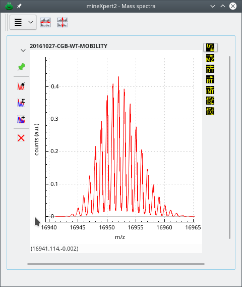
Calculated isotopic cluster for the monoprotonated apomyoglobin protein.
Figure 5.1: Calculation of the isotopic cluster of an analyte #
mineXpert2 provides an interface to the libIsoSpec++ library.
IsoSpec: Hyperfast Fine Structure Calculator
Mateusz K. Łącki, Michał Startek, Dirk Valkenborg, and Anna Gambin
Analytical Chemistry, 2017, 89, 3272–3277
DOI: 10.1021/acs.analchem.6b01459
This library performs high-resolution isotopic cluster calculations. In order to run the calculations, it is necessary to have the following items ready:
An elemental composition formula of the analyte (for example, H2O1). This formula needs to account for the ionization agent that is involved in the ionization of the analyte prior to its detection in the mass spectrometer.

Important
The IsoSpec software requires that all the chemical elements of a chemical formula be indexed. This means that, for water, for example, the formula should be H2O1 (notice the index 1 after the O element symbol).
A detailed isotopic configuration of all the chemical elements that are used in the elemental composition formula. mineXpert2 provides two interfaces to define the isotopic characteristics of the chemical elements. These will be described in the following sections.
5.1.1 The IsoSpec Graphical User Interface in mineXpert #
Generating iosotopic clusters using the IsoSpec software package is not easily carried over, in particular because this remarkable library is designed to be highly performant. The authors rightfully put their energy into optimizations for accuracy and speed instead of investing in a graphical user interface. mineXpert2 provides that graphical user interface, shown in Figure 5.2, “Isotopic cluster calculation dialog window”, that shows up upon selection of the program's main window's → menu.
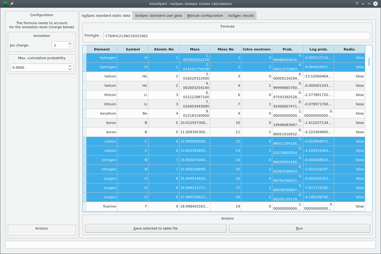
The dialog window contains two panels. The left hand side panel configures the charge for which the calculation is to be carried over and the maximum cumulative isotopic presence probability that IsoSpec must reach during the calculation. The right hand side panel contains a tab widget that contains the configuration tabs and the results tab.
Figure 5.2: Isotopic cluster calculation dialog window #
An isotopic cluster calculation is most probably performed with the aim of simulating an expected isotopic cluster for an analyte that is being analyzed by mass spectrometry. It is thus logical that the analyte be in an ionized form. The way that the analyte has been ionized needs to be taken into account in the chemical formula that describes the ion for which the isotopic cluster is being calculated. For example, when determining the chemical formula of a protein in the positive ion mode, the number of protons used to ionize the protein need to be included in the analyte elemental composition formula.
Warning
The IsoSpec software is “charge-agnostic” in the sense that it does not know what element in the chemical formula is responsible for the ionization of the analyte. Therefore, IsoSpec does not know of (and does not care about) the charge of the analyte. The ionization level of the analyte can be handled by mineXpert2 if that information is set to the Ion charge spin box widget. By default, the charge state of the analyte is 1.
The Max. cumulative probability spin box widget serves to configure the extent to which IsoSpec simulates the theoretically expected isotopic cluster. A value of 0.99 tells the software to simulate enough combinations of the analyte isotopes to represent 99 % of the theoretically expected combinations.
Tip
For large biopolymers, it might be prudent to start with a relatively low value for Max. cumulative probability, because setting this value too high, that is, near 1, would increase notably the calculation duration.
To perform isotopic cluster calculations, the simulation software needs to be aware of all the isotopes of all the chemical elements that enter in the composition of the ionized analyte. An isotope is defined by its mass and by the probability that it is found in nature. Carbon has two major isotopes that can be found in nature: the [12C] most abundant isotope and the [13C] least abundant isotope (the [14C] isotope is irrelevant for conventional mass spectrometry unless molecules have been artificially enriched in that isotope).
There are three ways that the user might use the IsoSpec software package. Two of them involve a configuration preparation on the part of the user. The third one, that we'll describe first, does not involve any chemical element configuration. The other ways are reviewed in the next sections.
5.1.1.1 Static Standard Element Tables Shipped within the IsoSpec Library #
In order to document all the chemical elements' isotopes' characteristics, the IsoSpec library has, in its own headers, a number of arrays that mineXpert2 automatically loads up when opening the Figure 5.2, “Isotopic cluster calculation dialog window” dialog window.[12] These data are displayed in the IsoSpec standard static data tab. The table view widget is not editable, hence the static qualifier in the tab name.
In this tab, all the user has to do is enter the formula for which the isotopic cluster calculation is to be performed. The formula needs to be pasted in the Formula line edit widget.
Once the formula has been set to its line edit widget, configure the charge of the ion (Ion charge spin box widget) and the Max. cumulative probability. Now, click .
5.1.1.2 Modified Standard Element Tables Shipped within the IsoSpec Library #
While the previous section showed how to use the static element tables from the IsoSpec library, this section shows a way to configure these elemental data. For this, start from the standard IsoSpec-based data and modify them according to one's needs. To proceed, select all the element rows of interest from the IsoSpec standard static data tab and click .
Tip
The order with which the rows are selected is respected in the export, so make sure to select the rows in the order that makes sense for you. Also, be sure to select rows and not only some cells; to achieve, this click in the left margin of the table view widget.
The export is performed as a text TSV (tab-separated value format) file in a layout that closely mimicks the data visible in the table view. Once the file has been saved, open it up in LibreOffice and modify the data to suit your needs. For example, in case of a labelling with [13C], with an efficiency of almost 98 %, lets's change the [12C] abundance (probability) to 0.02 and the [13C] abundance to 0.98.
Now that the modifications were performed, save the file under the same format and load it in the IsoSpec standard user data tab of the dialog window by clicking Load table from file. The table view now shows the new carbon abundance values. From now on, use this tab exactly like you did for the standard isospec static data work described above.
Here also, it is possible to select determinate rows and then save them to a file for later use.
5.1.1.3 User hand-made configuration of the element data within mineXpert #
The last way the user might configure the chemical elements to be used during an isotopic cluster calculation is based on the fully manual description of the elements and of the isotopes. That configuration is performed in the Manual configuration tab of the dialog window. This method is slightly more involved than the previous one but provides also for a much greater flexibility: it allows one to create “new chemical elements” that might be required in specific labelling experiments. The manual configuration is carried over in the Manual configuration tab of the dialog, as shown in Figure 5.3, “Hand-made user configuration of the chemical elements and formula”.
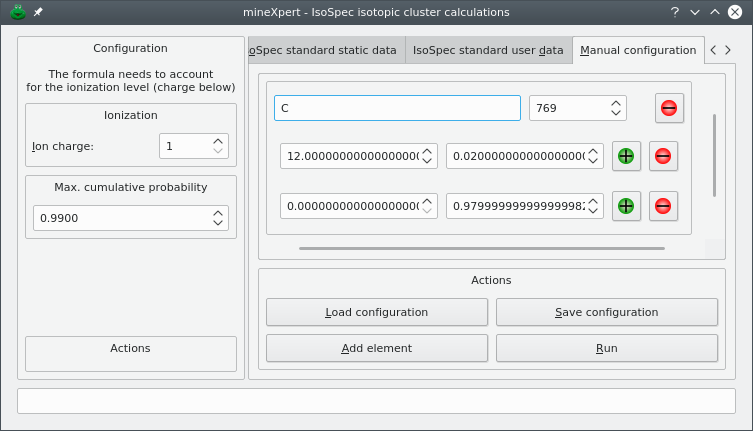
When the dialog is created, the tab is empty. To start creating element definitions, click .
Figure 5.3: Hand-made user configuration of the chemical elements and formula #
Upon creation of the dialog window, the Manual configuration tab is empty, with only two rows of buttons at the bottom of the tab. To start configuring chemical elements, click to create an “element group box” that contains a number of widgets organized in two rows:
Top row, a line edit widget to receive the chemical element symbol, C in the example;
A spin box widget in which to set the number of such atoms in the formula for which the isotopic cluster is being calculated. In the example, we set this value to 769;
A button with a “minus” image that removes all the “element group box” in one go;
The bottom row contains an “isotope frame widget” with two spin boxes for the mass of the isotope being configured (left) and its corresponding abundance (right);
In addition to the spin boxes, two buttons, with a “plus” or a “minus” figure, allow one to respectively add or remove isotope frames.

Note
It is not possible to remove all the isotope frames from an element group box, otherwise that group box would become useless.
Once an isotope frame has been filled-up, a new line might be required. To create a new isotope frame widget, click any “plus”-labelled button in any of the isotope frames. Once a new frame is created, the spin box widgets that it contains are set to 0.00000. Fill-in these spin boxes with mass and abundance and go on along this path to create as many isotopes as required.
Once all the isotopes for a given chemical element have been defined, a new element might be needed. For this, click and start the configuration of the new element as described above.
The manual isotopic configuration of the chemical elements required to perform an isotopic cluster calculation for a given formula is tedious. The user may want to save a given configuration to a file (click Save configuration) so that it is easier to recreate automatically all the widgets upon loading of that saved configuration (click Load configuration).
The final configuration is shown in Figure 5.4, “Typical manual configuration of the isotopic characteristics of the chemical elements”. The experiment that was configured above is a labelling of a glucose molecule with Cz, an imaginary chemical element that is like carbon but that has a [14C]. The glucose molecule (normal formula: C6H12O6) is labelled on one single carbon atom with an efficieny of 95 %. This means that, when the labelling fails (in 5 % of the cases) the carbon atom has its isotopes with usual probabilities (compounded by the fact that the normal atom is found at that position only in 5 % of the cases). The isotopic abundances for the Cz element are thus:
For [12C]: 0.05 * normal [12C] abundance;
For [13C]: 0.05 * normal [13C] abundance;
For [14C]: 0.95;
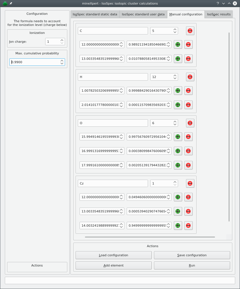
The user has configured a labelling experiment where the glucose molecule is labelled at a single carbon position with a [14C] atom (the efficiency of the labelling is 95 %).
Figure 5.4: Typical manual configuration of the isotopic characteristics of the chemical elements #
Note
Note that the “normal” carbon count is 5 (and not 6), that the hydrogen count is 13 (and not 12, because the glucose is protonated) and the labelled carbon is present only once.
5.1.1.4 The IsoSpec results are not shaped mass peaks #
Once the configurations have been terminated, the calculations can finally be performed by the IsoSpec library. In the manual configuration setting, the formula is automatically handled since each chemical element that is defined goes along with the count of the correponding atoms. In the case of the standard IsoSpec configuration (either modified or not), the user has to enter the chemical formula of the analyte in the Formula line edit widget.
Click Run. If the configuration was correct and IsoSpec could run the calculation properly, then the dialog window switches to the IsoSpec results tab (Figure 5.5, “Results from the isotopic cluster calculation”). That tab contains a text edit widget in which the results are displayed.
Note that the m/z values calculated by IsoSpec are “corrected” for the charge level that was specified in the left panel of the dialog window prior to their display in the results tab (Figure 5.2, “Isotopic cluster calculation dialog window”).
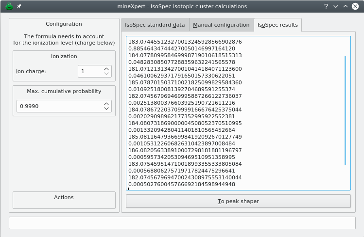
The IsoSpec library computes the probability of the various combinations of all the isotopes that make the chemical formula submitted to it. The results are in the form of peak centroid values along with corresponding probabilities. The sum of the probabilities corresponds to the Max. cumulative probability value that was set by the user.
Figure 5.5: Results from the isotopic cluster calculation #
The results that are produced by IsoSpec represent the peak centroids of the isotopic cluster. The results are thus a set of (m/z,i) pairs that have not the characteristic shape (the profile) that is found in mass spectra. mineXpert2 features the ability to give a shape to the centroid peaks. For that, click To peak shaper to open the Peak Shaper dialog window preloaded with the IsoSpec-generated peak centroids. The workings of this peak shaping feature is described in Section 5.2, “Shaping mass peak centroids into well-profiled peaks”.
5.2 Shaping mass peak centroids into well-profiled peaks #
The shape of mass peaks is typically Gaussian or Lorentzian (or a mix thereof). There are some data simulation or analysis processes that lead to having mass peaks characterized by a single centroid m/z value and a corresponding intensity. Plotted to a graph, a centroid mass peak yields a bar. In order to convert mass peak centroids into something that resembles a real “profile” mass peaks, a mathematical formula can be applied, with some parameters to configure the shapes generated. mineXpert2 includes that feature, accessible via the → menu item. The window that opens up is shown in Figure 5.6, “Setting-up of the centroid mass peak shaping process”
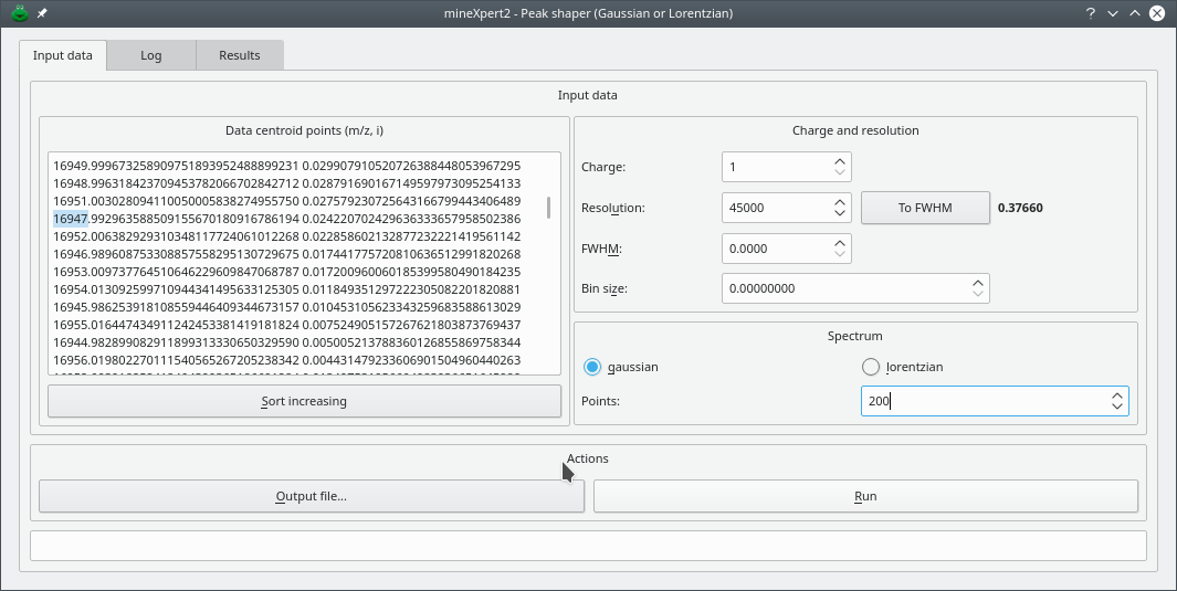
This dialog window allows one to configure the shaping of mass centroid peaks. Setting a spectrum name in the Mass spectrum name line edit widget will help recognize the result mass spectrum once displayed in the Mass spectra window (see below).
Figure 5.6: Setting-up of the centroid mass peak shaping process #
The mass centroid peaks are listed in the Data centroid points (m/z,i) text edit widget. These values are pasted there by the user or copied automatically from the isotopic cluster calculation dialog window (see Section 5.1.1.4, “The IsoSpec results are not shaped mass peaks”). The width of the “profile” mass peak is determined either by setting the resolution of the instrument (in the example, that is set to 45000) or by setting the width of the peak at half maximum of its height (FWHM).
The spectrum that is generated can be of a Gaussian or a Lorentzian shape. That parameter is configured by selecting the corresponding radio button widget. The number of points used to actually craft the shape of the peak is configurable. In the example, that parameter is set to 200.
Tip
When defining the parameters for the peak shaping process, it might be useful to have and idea of the FWHM value at a given m/z value for a given resolution. To compute that FWHMvalue, double-click-select a single mass peak centroid m/z value from the text edit widget, set the resolving power of your instrument and then click . The computed FWHM value will be displayed next to the button. The text is selectable so as to copy it to the clipboard and then in the FWHM spin box widget.
Once the peak shaping parameters have been set, click . The dialog window shifts tab to Results, as shown in Figure 5.7, “Shaped peaks mass spectral data”.
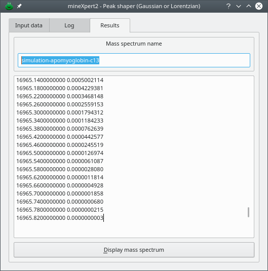
The mass spectral data corresponding to the combination of each individual “peak-shaped” centroid peak are displayed in this tab. Plotting these data will produce a nicely shaped isotopic cluster matching what would be seen by recording a mass spectrum on an instrument.
Figure 5.7: Shaped peaks mass spectral data #
Tip
To ensure that various isotopic cluster calculation-based mass spectra can later be recognized, the user is advised, for the different simulations, to insert distinct names in the Mass spectrum name line edit widget. This name will be used later when creating the mass spectrum if the user asks that the mass spectrum be displayed by clicking . In the eventuality that the mass spectrum name is not changed from a simulation to the other, a safeguard process ensures that names are absolutely unambiguous by appending to the mass spectrum name the time at which the mass spectrum is displayed.
It is possible to automatically plot the result mass spectrum by clicking . The process gets a little involved here because the mass spectrum is not created from a file, and mineXpert2's handling of plots is based on the fact that a MS run data set has been created, typically at data file loading time. Two situations may arise:
If not a single MS run data set is currently available (that is, no single mass spectrometry data file was loaded during the current session), the program will inform the user that a shim MS run data set was created (Figure 5.8, “Creation of a shim MS run data set”). At this time, the dialog window listing all the open MS run data sets will show up (Figure 2.2, “The open MS run data sets”). The information message advises to perform the task again, that is, click .
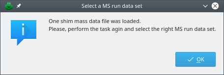
This information dialog window informs the user that a new shim MS run data set was created. Shim MS run data sets need to be created when new plots are created for data that were not loaded from a disk file. The user is advised to repeat the last action. In this case, click again. The next step is described in the text below.
Figure 5.8: Creation of a shim MS run data set #
If at least one MS run data set was loaded already in the program, then an input dialog window shows up letting the user select the MS run data set to which the isotopic cluster calculation mass spectrum is to be anchored to (Figure 5.9, “Selection of a MS run data set”). It is always possible to ask that a new MS run data set be created ex nihilo for the new mass spectrum by selecting Create a new MS run data set. In this case, the process goes back to the previous item. This process is useful if each mass spectrum must have a distinct color.
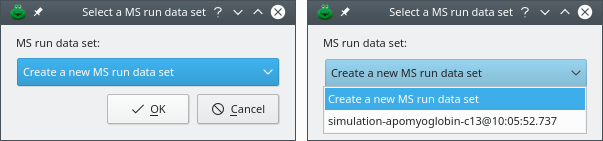
If one or more MS run data set(s) preexisted in the program, this input dialog shows up (left). Upon clicking the combo box widget, the user can select the MS run data set to anchor the new mass spectrum to (right).
Figure 5.9: Selection of a MS run data set #
The isotopic cluster calculation-based mass spectrum shows up in the Mass spectra window, as shown in Figure 5.10, “Spectrum created using the peak shaping feature”.
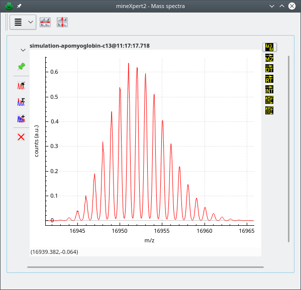
The spectrum corresponds to a combination of each individual spectrum obtained by shaping each individual mass peak centroid in the input data list.
Figure 5.10: Spectrum created using the peak shaping feature #
Note that if the resolution asked is very high, the resulting shaped mass peaks might appear a bit “hairy”. By tweaking the Bin size value, the binning of the spectra might improve the situation. Otherwise, using the plot widget main menu to apply a Savitzky-Golay filter, described at Section 3.1.6, “Savitzky-Golay filtering of any kind of data”, will certainly improve things.
Tip
If the peak centroids were not “corrected” for their charge in the previous generation step (as in the case of the isotopic cluster calculation, it is still time to apply this “correction” by setting the charge in the Charge spin box widget. If the charge was already accounted for, as described in Section 5.1.1.4, “The IsoSpec results are not shaped mass peaks”, then leave the charge to 1 and the results will be correct.